About Me

Junna Yanai Bibliography
My name is Junna Yanai and I am from the San Francisco Bay Area. I was born in Japan, studied in the U.S.A. until high school, and graduated from dual degree between Sciences Po Paris and Keio University for a Bachelors in Economics. I am very excited to attend London Business School.

My hobbies are:
- running
- tennis
- baking
- taking photos of flowers and puppies
Please take a look at my Linkedin: Linkedin Link
Please take a look at my CV: CV
Below are some of the basics analysis that I have done in my Master’s program:
Gapminder Analysis
glimpse(gapminder)## Rows: 1,704
## Columns: 6
## $ country <fct> "Afghanistan", "Afghanistan", "Afghanistan", "Afghanistan", …
## $ continent <fct> Asia, Asia, Asia, Asia, Asia, Asia, Asia, Asia, Asia, Asia, …
## $ year <int> 1952, 1957, 1962, 1967, 1972, 1977, 1982, 1987, 1992, 1997, …
## $ lifeExp <dbl> 28.801, 30.332, 31.997, 34.020, 36.088, 38.438, 39.854, 40.8…
## $ pop <int> 8425333, 9240934, 10267083, 11537966, 13079460, 14880372, 12…
## $ gdpPercap <dbl> 779.4453, 820.8530, 853.1007, 836.1971, 739.9811, 786.1134, …head(gapminder, 20) # look at the first 20 rows of the dataframe## # A tibble: 20 × 6
## country continent year lifeExp pop gdpPercap
## <fct> <fct> <int> <dbl> <int> <dbl>
## 1 Afghanistan Asia 1952 28.8 8425333 779.
## 2 Afghanistan Asia 1957 30.3 9240934 821.
## 3 Afghanistan Asia 1962 32.0 10267083 853.
## 4 Afghanistan Asia 1967 34.0 11537966 836.
## 5 Afghanistan Asia 1972 36.1 13079460 740.
## 6 Afghanistan Asia 1977 38.4 14880372 786.
## 7 Afghanistan Asia 1982 39.9 12881816 978.
## 8 Afghanistan Asia 1987 40.8 13867957 852.
## 9 Afghanistan Asia 1992 41.7 16317921 649.
## 10 Afghanistan Asia 1997 41.8 22227415 635.
## 11 Afghanistan Asia 2002 42.1 25268405 727.
## 12 Afghanistan Asia 2007 43.8 31889923 975.
## 13 Albania Europe 1952 55.2 1282697 1601.
## 14 Albania Europe 1957 59.3 1476505 1942.
## 15 Albania Europe 1962 64.8 1728137 2313.
## 16 Albania Europe 1967 66.2 1984060 2760.
## 17 Albania Europe 1972 67.7 2263554 3313.
## 18 Albania Europe 1977 68.9 2509048 3533.
## 19 Albania Europe 1982 70.4 2780097 3631.
## 20 Albania Europe 1987 72 3075321 3739.Country data and continent data
country_data <- gapminder %>%
            filter(country == "Japan")

continent_data <- gapminder %>%
            filter(continent == "Asia")
Country (Japan) life expectency
plot1 <- ggplot(data = country_data, mapping = aes(x = year, y = lifeExp))+
   geom_point() +
   geom_smooth(se = FALSE)+
  NULL
plot1
## `geom_smooth()` using method = 'loess' and formula 'y ~ x'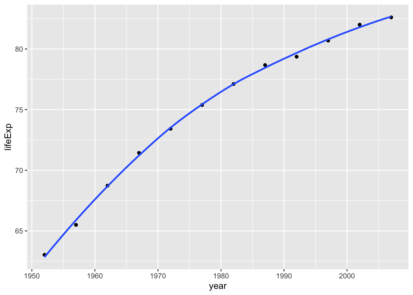
Entering the title and axes
 plot1<- plot1 +
   labs(title = "Japan Life Expectancy",
       x = "Year",
       y = "Life Expectancy") +
   NULL


 plot1
## `geom_smooth()` using method = 'loess' and formula 'y ~ x'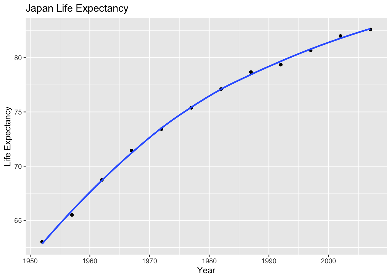
In Japan, the life expectancy has grown significantly since the 1950s as it become an industrial developed nation. This is because Japan experienced high death rates and low living standards during wartime but now is one of the most medically advanced countries in the world.
Life expectancy in Asia
 ggplot(continent_data, mapping = aes(x =year , y =lifeExp  , colour= country, group = country))+
   geom_point() +
   geom_smooth(se = FALSE) +
   NULL
## `geom_smooth()` using method = 'loess' and formula 'y ~ x'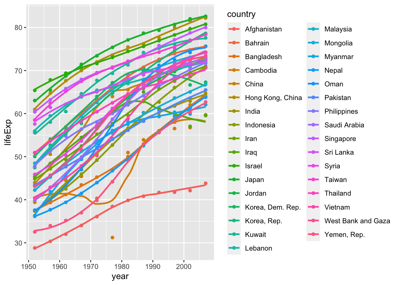
We can see from this graph that the life expectancy is on an upward trend in every country in Asia. This is because the living standards and health of individuals in these countries are improving as the countries become more developed.
World life expectancy by continent
 ggplot(data = gapminder , mapping = aes(x = year , y = lifeExp , colour= continent))+
   geom_point() +
   geom_smooth(se = FALSE) +
   facet_wrap(~continent) +
   theme(legend.position="none") + #remove all legends
   NULL
## `geom_smooth()` using method = 'loess' and formula 'y ~ x'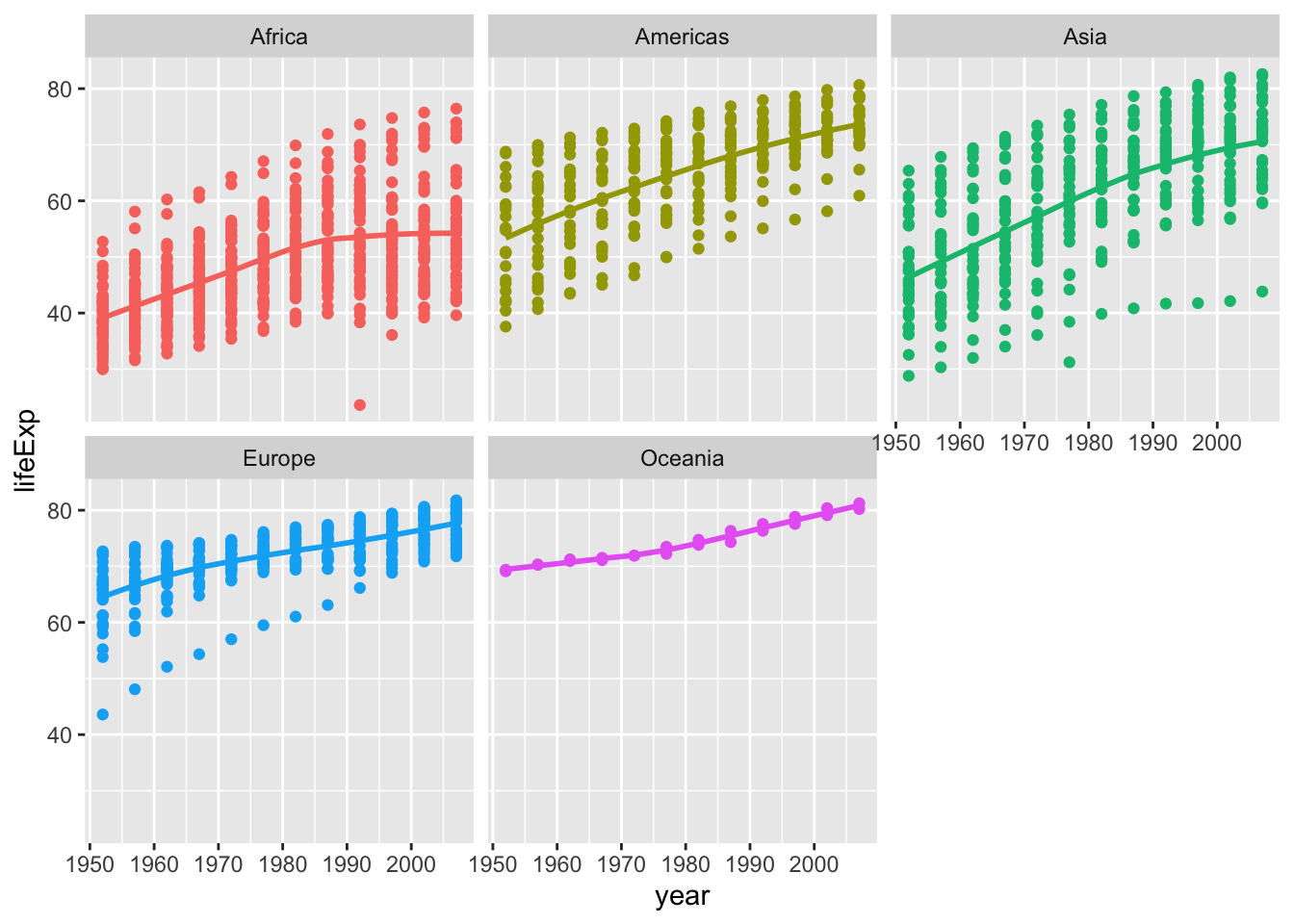
Life expectancy is increasing in all parts of the world. Asian countries like Japan and Korea tend to have higher life expectancy compared to other countries throughout the years, and the average stands around 80 years old. The reason why these countries tend to have higher life expectencies is supposedly due to healthier diet and lack of patients from diseases like heart disease which are caused from obesity. People from western countries tend to suffer from such health problems, and people from poor countries lack access to healthcare.
Brexit vote analysis
Brexit data
brexit_results <- read_csv(here::here("data","brexit_results.csv"))


glimpse(brexit_results)
## Rows: 632
## Columns: 11
## $ Seat <chr> "Aldershot", "Aldridge-Brownhills", "Altrincham and Sale W…
## $ con_2015 <dbl> 50.592, 52.050, 52.994, 43.979, 60.788, 22.418, 52.454, 22…
## $ lab_2015 <dbl> 18.333, 22.369, 26.686, 34.781, 11.197, 41.022, 18.441, 49…
## $ ld_2015 <dbl> 8.824, 3.367, 8.383, 2.975, 7.192, 14.828, 5.984, 2.423, 1…
## $ ukip_2015 <dbl> 17.867, 19.624, 8.011, 15.887, 14.438, 21.409, 18.821, 21.…
## $ leave_share <dbl> 57.89777, 67.79635, 38.58780, 65.29912, 49.70111, 70.47289…
## $ born_in_uk <dbl> 83.10464, 96.12207, 90.48566, 97.30437, 93.33793, 96.96214…
## $ male <dbl> 49.89896, 48.92951, 48.90621, 49.21657, 48.00189, 49.17185…
## $ unemployed <dbl> 3.637000, 4.553607, 3.039963, 4.261173, 2.468100, 4.742731…
## $ degree <dbl> 13.870661, 9.974114, 28.600135, 9.336294, 18.775591, 6.085…
## $ age_18to24 <dbl> 9.406093, 7.325850, 6.437453, 7.747801, 5.734730, 8.209863…Distribution of leave % in all constituencies
# histogram
ggplot(brexit_results, aes(x = leave_share)) +
  geom_histogram(binwidth = 2.5)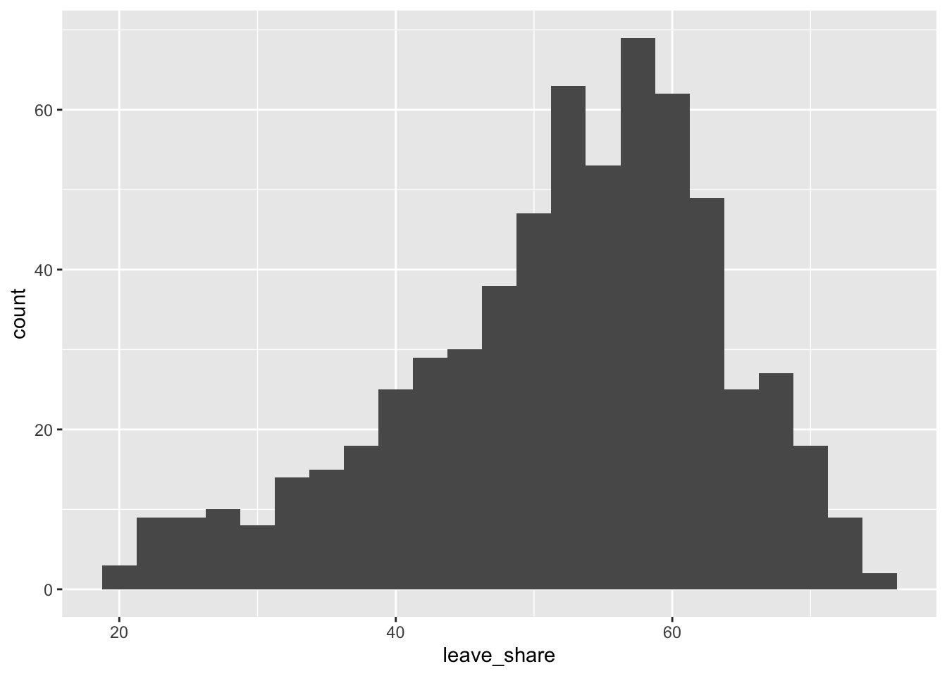
# density plot-- think smoothed histogram
ggplot(brexit_results, aes(x = leave_share)) +
  geom_density()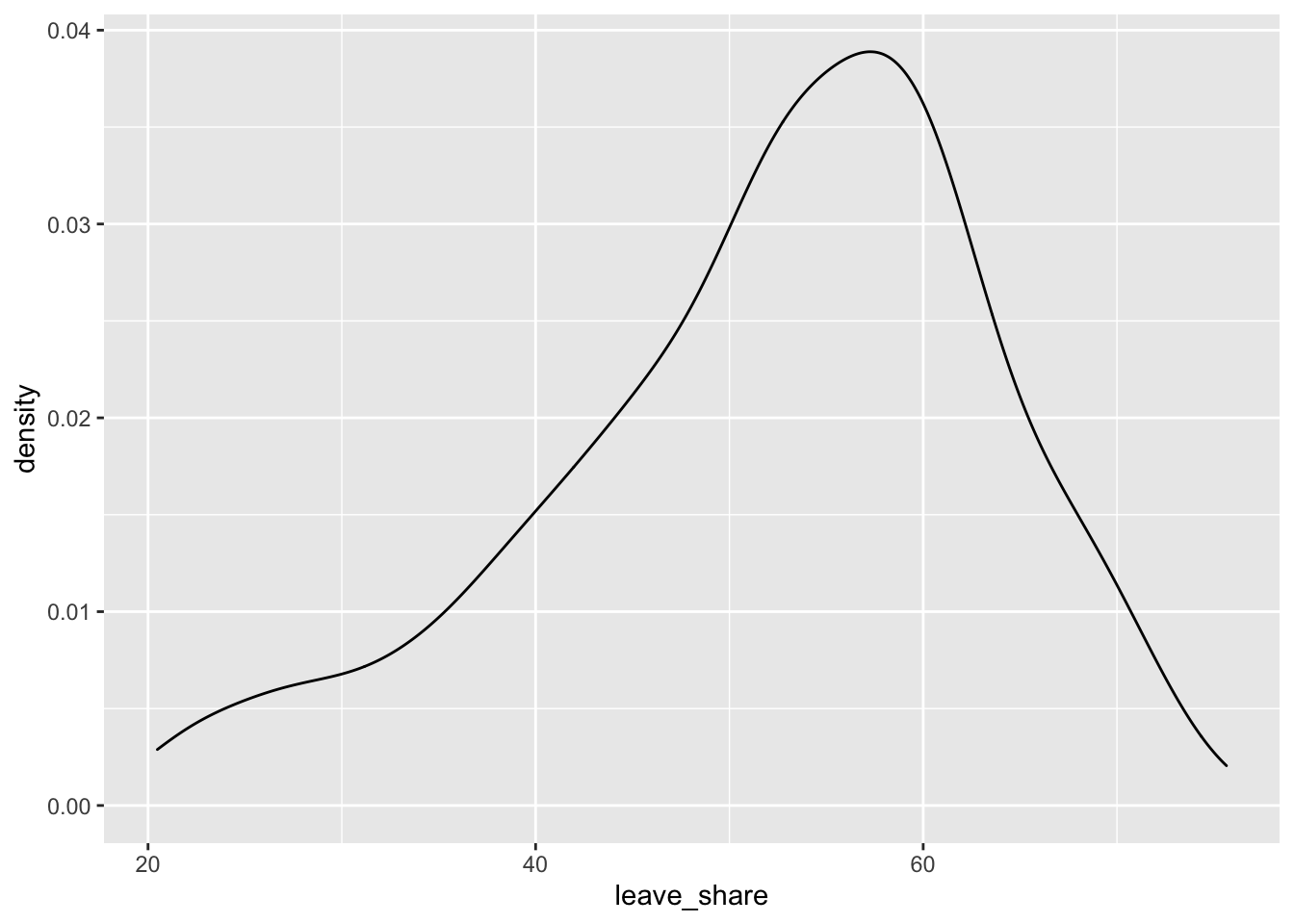
# The empirical cumulative distribution function (ECDF)
ggplot(brexit_results, aes(x = leave_share)) +
  stat_ecdf(geom = "step", pad = FALSE) +
  scale_y_continuous(labels = scales::percent)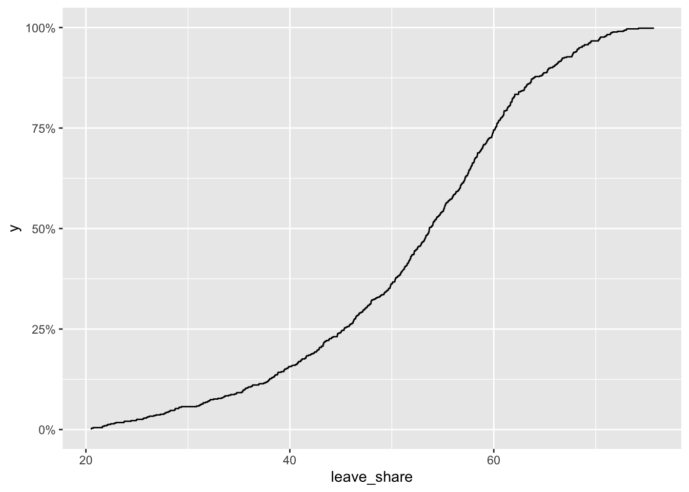
Scatterplot between leaveshare and born in UK
ggplot(brexit_results, aes(x = born_in_uk, y = leave_share)) +
  geom_point(alpha=0.3) +

  # add a smoothing line, and use method="lm" to get the best straight-line
  geom_smooth(method = "lm") +

  # use a white background and frame the plot with a black box
  theme_bw() +
  NULL
## `geom_smooth()` using formula 'y ~ x'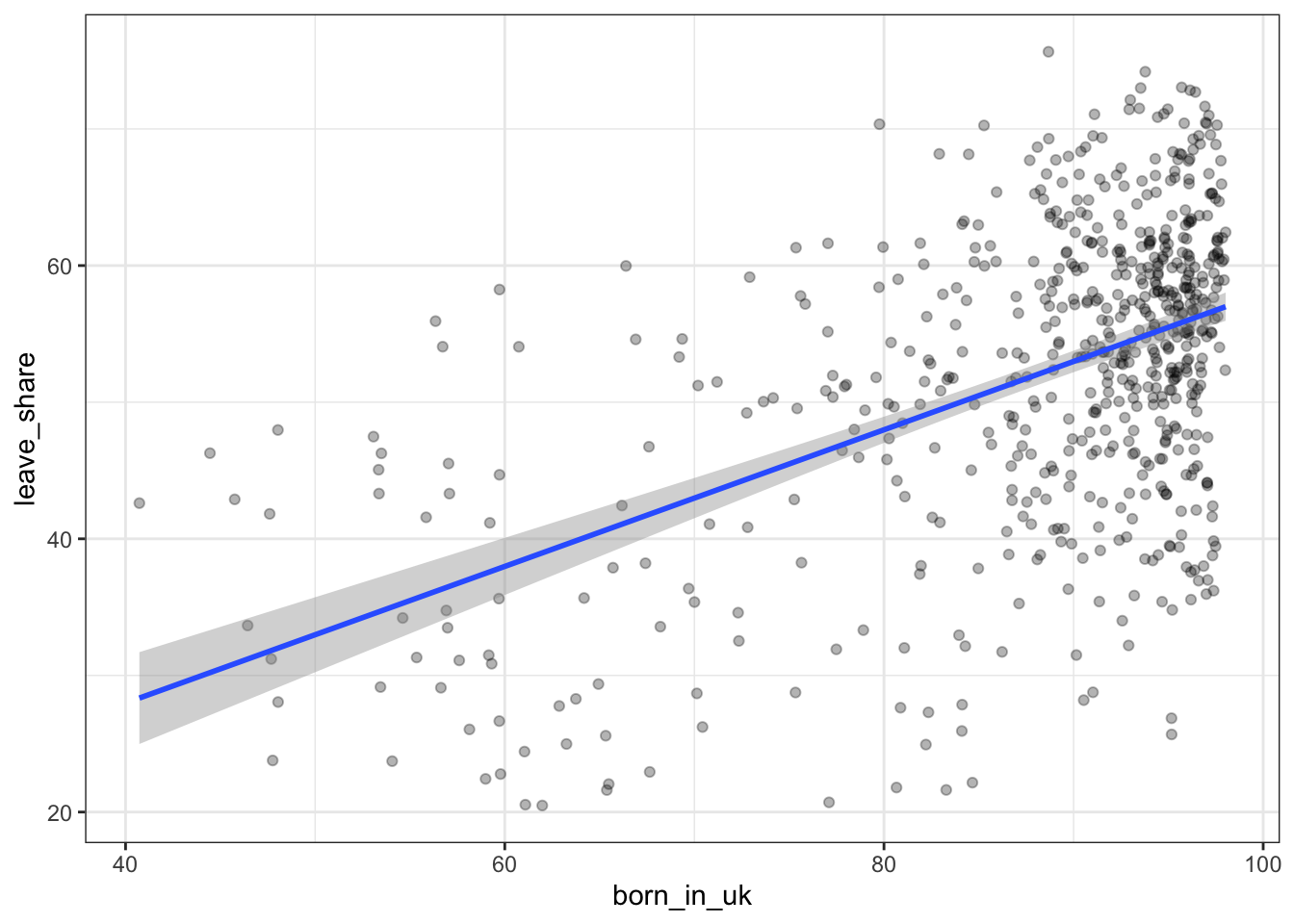
The correlation between individuals born in the UK who have voted to leave the EU is high. Individuals who are born in the UK are UK citizens who have not immigrated to live in the country, hence their mentality towards the EU and the ease of currency exchange and immigration, as well as lack of flexibility for individual member countries for policy and public financing contributed to UK born citizens voting to leave the UK at higher rates that other groups.
Animal rescue incidents attended by the London Fire Brigade
Data on animal rescue
url <- "https://data.london.gov.uk/download/animal-rescue-incidents-attended-by-lfb/8a7d91c2-9aec-4bde-937a-3998f4717cd8/Animal%20Rescue%20incidents%20attended%20by%20LFB%20from%20Jan%202009.csv"

animal_rescue <- read_csv(url,
                          locale = locale(encoding = "CP1252")) %>%
  janitor::clean_names()


glimpse(animal_rescue)
## Rows: 7,772
## Columns: 31
## $ incident_number <chr> "139091", "275091", "2075091", "2872091"…
## $ date_time_of_call <chr> "01/01/2009 03:01", "01/01/2009 08:51", …
## $ cal_year <dbl> 2009, 2009, 2009, 2009, 2009, 2009, 2009…
## $ fin_year <chr> "2008/09", "2008/09", "2008/09", "2008/0…
## $ type_of_incident <chr> "Special Service", "Special Service", "S…
## $ pump_count <chr> "1", "1", "1", "1", "1", "1", "1", "1", …
## $ pump_hours_total <chr> "2", "1", "1", "1", "1", "1", "1", "1", …
## $ hourly_notional_cost <dbl> 255, 255, 255, 255, 255, 255, 255, 255, …
## $ incident_notional_cost <chr> "510", "255", "255", "255", "255", "255"…
## $ final_description <chr> "Redacted", "Redacted", "Redacted", "Red…
## $ animal_group_parent <chr> "Dog", "Fox", "Dog", "Horse", "Rabbit", …
## $ originof_call <chr> "Person (land line)", "Person (land line…
## $ property_type <chr> "House - single occupancy", "Railings", …
## $ property_category <chr> "Dwelling", "Outdoor Structure", "Outdoo…
## $ special_service_type_category <chr> "Other animal assistance", "Other animal…
## $ special_service_type <chr> "Animal assistance involving livestock -…
## $ ward_code <chr> "E05011467", "E05000169", "E05000558", "…
## $ ward <chr> "Crystal Palace & Upper Norwood", "Woods…
## $ borough_code <chr> "E09000008", "E09000008", "E09000029", "…
## $ borough <chr> "Croydon", "Croydon", "Sutton", "Hilling…
## $ stn_ground_name <chr> "Norbury", "Woodside", "Wallington", "Ru…
## $ uprn <chr> "NULL", "NULL", "NULL", "100021491149", …
## $ street <chr> "Waddington Way", "Grasmere Road", "Mill…
## $ usrn <chr> "20500146", "NULL", "NULL", "21401484", …
## $ postcode_district <chr> "SE19", "SE25", "SM5", "UB9", "RM3", "RM…
## $ easting_m <chr> "NULL", "534785", "528041", "504689", "N…
## $ northing_m <chr> "NULL", "167546", "164923", "190685", "N…
## $ easting_rounded <dbl> 532350, 534750, 528050, 504650, 554650, …
## $ northing_rounded <dbl> 170050, 167550, 164950, 190650, 192350, …
## $ latitude <chr> "NULL", "51.39095371", "51.36894086", "5…
## $ longitude <chr> "NULL", "-0.064166887", "-0.161985191", …Animal rescue count
animal_rescue %>%
  dplyr::group_by(cal_year) %>%
  summarise(count=n())
## # A tibble: 13 × 2
## cal_year count
## <dbl> <int>
## 1 2009 568
## 2 2010 611
## 3 2011 620
## 4 2012 603
## 5 2013 585
## 6 2014 583
## 7 2015 540
## 8 2016 604
## 9 2017 539
## 10 2018 610
## 11 2019 604
## 12 2020 758
## 13 2021 547animal_rescue %>%
count(cal_year, name="count")## # A tibble: 13 × 2
## cal_year count
## <dbl> <int>
## 1 2009 568
## 2 2010 611
## 3 2011 620
## 4 2012 603
## 5 2013 585
## 6 2014 583
## 7 2015 540
## 8 2016 604
## 9 2017 539
## 10 2018 610
## 11 2019 604
## 12 2020 758
## 13 2021 547There is no evident trend for the number of animal incident count, as seen above.
Animal Group Percentages
animal_rescue %>%
  group_by(animal_group_parent) %>%

  #group_by and summarise will produce a new column with the count in each animal group
  summarise(count = n()) %>%

  # mutate adds a new column; here we calculate the percentage
  mutate(percent = round(100*count/sum(count),2)) %>%

  # arrange() sorts the data by percent. Since the default sorting is min to max and we would like to see it sorted
  # in descending order (max to min), we use arrange(desc())
  arrange(desc(percent))
## # A tibble: 28 × 3
## animal_group_parent count percent
## <chr> <int> <dbl>
## 1 Cat 3736 48.1
## 2 Bird 1611 20.7
## 3 Dog 1213 15.6
## 4 Fox 366 4.71
## 5 Unknown - Domestic Animal Or Pet 199 2.56
## 6 Horse 195 2.51
## 7 Deer 132 1.7
## 8 Unknown - Wild Animal 93 1.2
## 9 Squirrel 66 0.85
## 10 Unknown - Heavy Livestock Animal 50 0.64
## # … with 18 more rowsanimal_rescue %>%
#count does the same thing as group_by and summarise
# name = "count" will call the column with the counts "count" ( exciting, I know)
# and 'sort=TRUE' will sort them from max to min
count(animal_group_parent, name="count", sort=TRUE) %>%
mutate(percent = round(100*count/sum(count),2))## # A tibble: 28 × 3
## animal_group_parent count percent
## <chr> <int> <dbl>
## 1 Cat 3736 48.1
## 2 Bird 1611 20.7
## 3 Dog 1213 15.6
## 4 Fox 366 4.71
## 5 Unknown - Domestic Animal Or Pet 199 2.56
## 6 Horse 195 2.51
## 7 Deer 132 1.7
## 8 Unknown - Wild Animal 93 1.2
## 9 Squirrel 66 0.85
## 10 Unknown - Heavy Livestock Animal 50 0.64
## # … with 18 more rowsAs we can see from the percentages above, cats are almost half of the animal incidents that happen in absolute numbers. This is most likely because they are freely roaming around neighborhoods where humans live. They are vulnerable to cars running them over.
Animal Rescue dataframe
# what type is variable incident_notional_cost from dataframe `animal_rescue`
typeof(animal_rescue$incident_notional_cost)
## [1] "character"# readr::parse_number() will convert any numerical values stored as characters into numbers
animal_rescue <- animal_rescue %>%
# we use mutate() to use the parse_number() function and overwrite the same variable
mutate(incident_notional_cost = parse_number(incident_notional_cost))
# incident_notional_cost from dataframe `animal_rescue` is now 'double' or numeric
typeof(animal_rescue$incident_notional_cost)## [1] "double"Summary statistics
animal_rescue %>%

  # group by animal_group_parent
  group_by(animal_group_parent) %>%

  # filter resulting data, so each group has at least 6 observations
  filter(n()>6) %>%

  # summarise() will collapse all values into 3 values: the mean, median, and count
  # we use na.rm=TRUE to make sure we remove any NAs, or cases where we do not have the incident cos
  summarise(mean_incident_cost = mean (incident_notional_cost, na.rm=TRUE),
            median_incident_cost = median (incident_notional_cost, na.rm=TRUE),
            sd_incident_cost = sd (incident_notional_cost, na.rm=TRUE),
            min_incident_cost = min (incident_notional_cost, na.rm=TRUE),
            max_incident_cost = max (incident_notional_cost, na.rm=TRUE),
            count = n()) %>%

  # sort the resulting data in descending order. You choose whether to sort by count or mean cost.
  arrange(desc(mean_incident_cost))
## # A tibble: 16 × 7
## animal_group_parent mean_incident_co… median_incident_… sd_incident_cost
## <chr> <dbl> <dbl> <dbl>
## 1 Horse 740. 596 541.
## 2 Cow 634. 520 475.
## 3 Deer 417. 333 286.
## 4 Unknown - Wild Animal 416. 333 324.
## 5 Unknown - Heavy Livesto… 374. 260 263.
## 6 Fox 373. 328 206.
## 7 Snake 356. 339 105.
## 8 Dog 347. 298 169.
## 9 Bird 344. 328 135.
## 10 Cat 343. 298 160.
## 11 Unknown - Domestic Anim… 326. 295 117.
## 12 cat 324. 290 94.1
## 13 Hamster 315. 290 95.0
## 14 Squirrel 313. 326 57.1
## 15 Ferret 309. 333 39.4
## 16 Rabbit 309. 326 32.2
## # … with 3 more variables: min_incident_cost <dbl>, max_incident_cost <dbl>,
## # count <int>First, I notice that the standard deviation is bigger for animals with higher incident costs and also that the median cost is clearly smaller than the mean costs. From this we can interpret that larger animals like horses, cows, and deers can get into accidents that can cost the most, but the price varied widely. This is not a surprise. In terms of outliers, we see that they mainly involve higher prices rather than lower prices. For instance, the maximum price for horse incidents is 3480, which is over 3 standard deviations away from the mean. Same goes for deers.
Plots on incident cost by animals group
# base_plot
base_plot <- animal_rescue %>%
  group_by(animal_group_parent) %>%
  filter(n()>6) %>%
  ggplot(aes(x=incident_notional_cost))+
  facet_wrap(~animal_group_parent, scales = "free")+
  theme_bw()

base_plot + geom_histogram()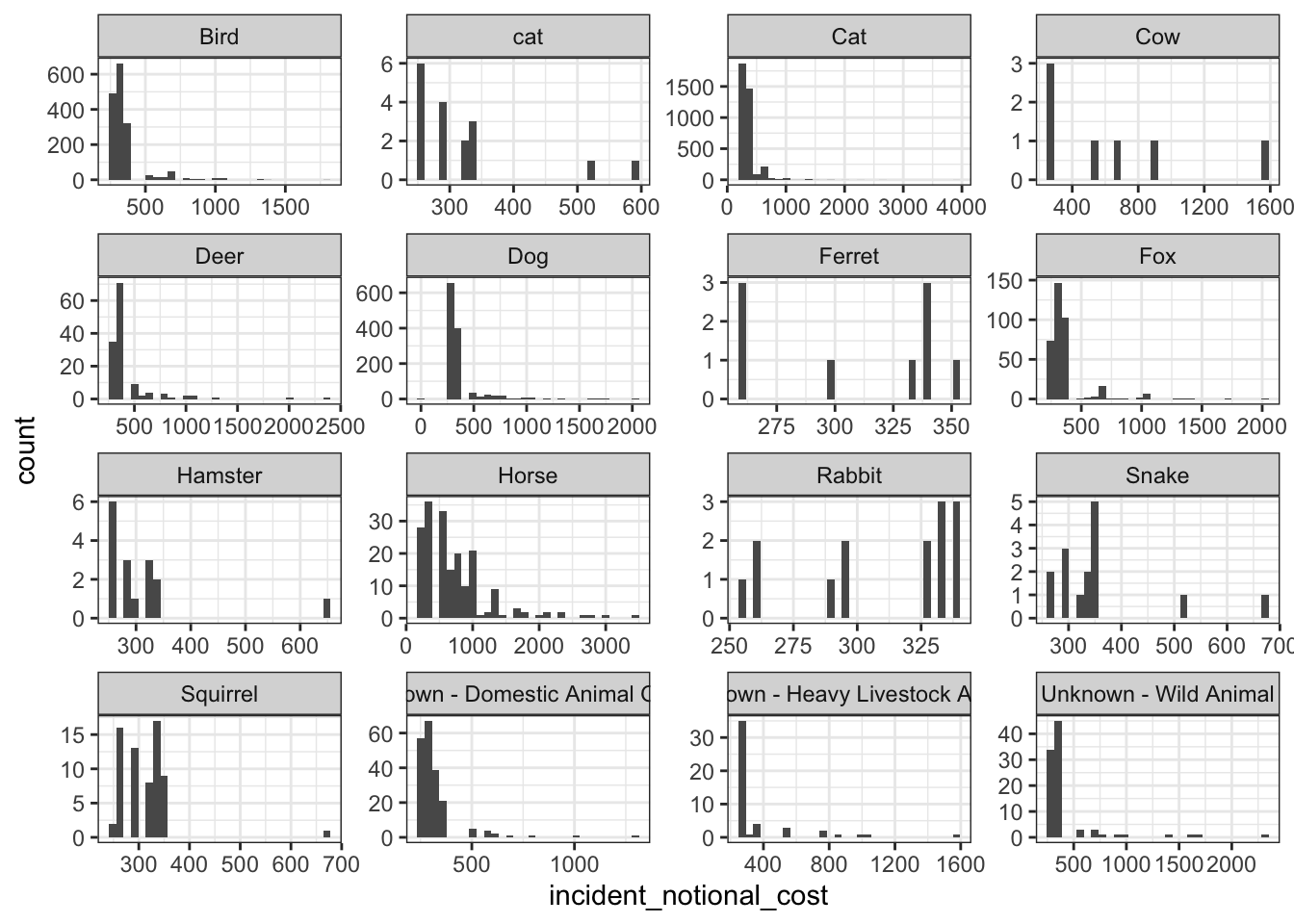
base_plot + geom_density()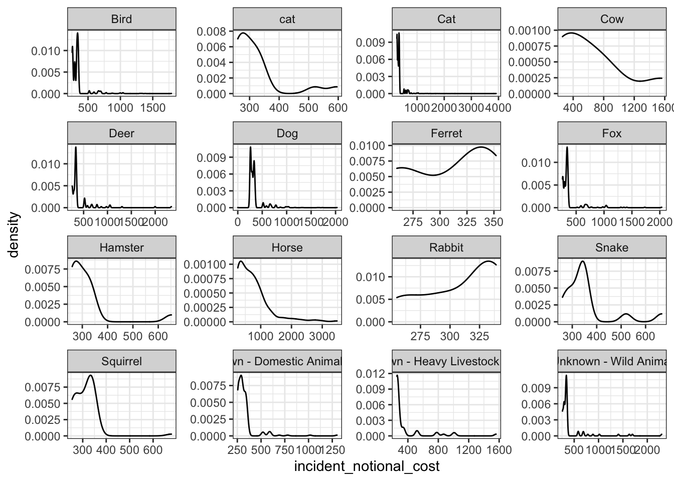
base_plot + geom_boxplot()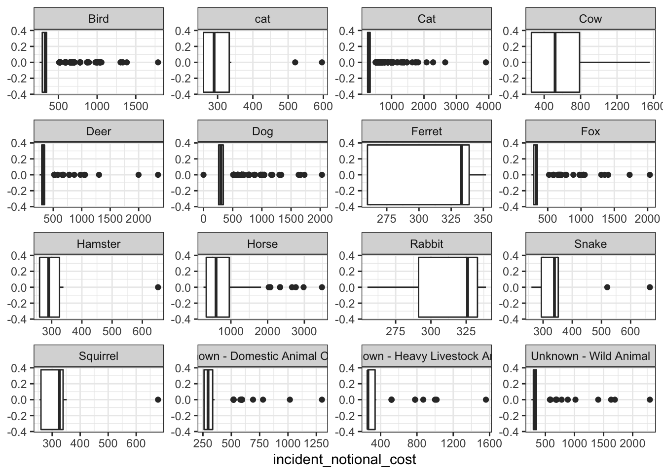
base_plot + stat_ecdf(geom = "step", pad = FALSE) +
  scale_y_continuous(labels = scales::percent)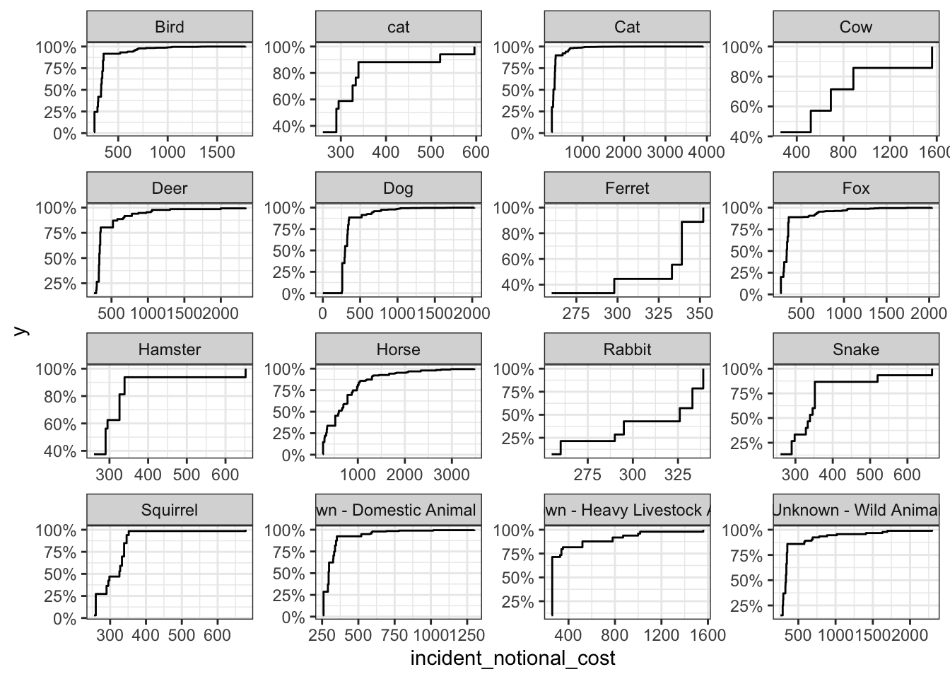
The histogram and box and whisker plot are most useful when communicating this information because it it clearly shows the distribution and the outliers. The line graph is more fit to represent data on continuous x values such as time. Based on the distribution of the above graphs, we can see that smaller rodent animals such as rabbits and ferrets have an even distribution that are less skewed compared to other animals. Animals such as horses and cows tend to be skewed to the right, with clear outliers for heavier incidents. However, these animals are still more expensive, as can be observed from the median values. This is most likely because they can cause larger impact at the incident scene as compared to smaller animals.